Energy Management in Smart-Grids on Example of a Washer-Dryer

This research and development project was funded by the German Federal Ministry of Education and Research (BMBF) within the Leading-Edge Cluster “Intelligent Technical Systems OstWestfalenLippe” (it ́s OWL) and managed by the Project Management Agency Karlsruhe (PTKA).
Project acronym: itsowl-EMWaTro
Funding period: 07/2013 - 09/2016
Project budget: 1,160,000 €
Project partner: Miele & Cie.
Project manager: PTKA
Motivation
In recent years, home automation has reached the end customer market enabling the customer to monitor and control the status of his consumers at home from a central location, and usually while on the move. This can also be done automatically using a ready-made scheme. However, since the systems do not have a control connection to the power grid, they are only isolated solutions for a single household. In addition, the systems lack optimization algorithms that independently and dynamically optimize the power requirements of the household depending on the situation.
Due to the advancing home automation, a wide range of control options for consumers in the household are already available today and will be available in the near future. With regard to load management and integration into a smart-grid, however, there is a lack of automatic interaction and dynamic cross-consumer optimization of generation and load profiles that is not based on static, time-of-day electricity tariffs.
Objectives
In the context of this project, the general conditions of a future smart-grid and the effects on private households had to be discussed first. On the basis of the results, a simulation system for a local network with detailing down to the device level was then to be created. In addition, an energy management system was to be developed and implemented in the simulation that optimally controls the operation of controllable devices in the local network. Finally, the function of the energy management system was to be validated by means of simulations.
General conditions and electricity tariffs
As direct interference in the operation of equipment could be perceived by private individuals as incapacitation, this option was discarded. Instead, a structure with offer and selection was applied. A time-variable tariff was chosen as an incentive for the postponement of loads. This tariff is generated from the stock exchange price and is already announced at noon for the following day.
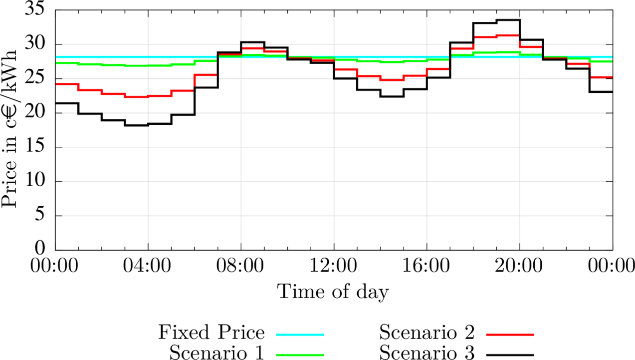
Since the current structure of the electricity price components means that more than 80 % of the price is accounted for by fixed absolute charges and levies, no significant price spread is to be expected if the generation costs, i.e. the exchange price, are purely dynamic. The red line in Fig. 1 shows the average resulting electricity tariff in light blue in comparison to the current tariff. In order to create a significant incentive, the price spread must be significantly increased. This can be done by coupling taxes and levies to the generation price and would be a revenue-neutral regulatory intervention by the legislator. This coupling would already result in a significant price spread, as the red curve in Fig. 1 shows. Assuming that in future distribution costs and grid fees, i.e. the money that goes to private companies, would also become more dynamic, we arrive at an average daily maximum price that is more than twice as high as the cheapest. In such a scenario, savings potentials of over 50 % would be achievable, which would provide a useful incentive to shift the load. The resulting average price trend is shown in the dark black curve in Fig. 1. The concrete values of the electricity price components (as of 2014) are shown in Tab. 1.
Price | 2014 c€/kWh | Dynamic Add-on |
Distribution | 4,23 | 81,87% |
Grid fees | 7,43 | 143,8% |
Taxes, Duties, Levies | 12,85 | 248,6% |
Tab. 1: Electricity Price Components 2014 and with Dynamisation
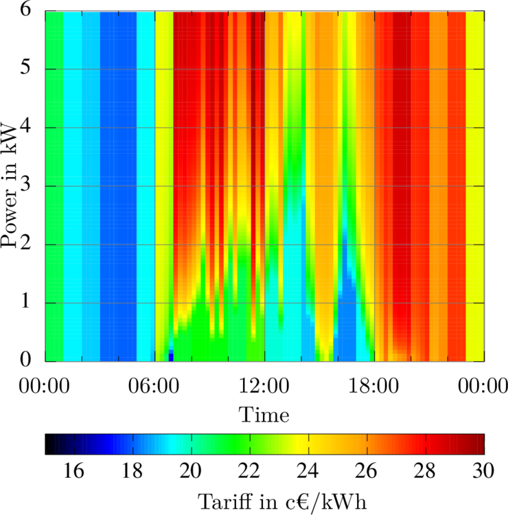
In addition to taking into account the generation capacity available in the grid via variable electricity tariffs, the project also took into account the own use of photovoltaics (PV) or other own electricity generation. It should be noted that the electricity generated by the own PV system is by no means free. This is not a matter of writing off an already existing plant, but of the feed-in tariffs for feeding electricity into the distribution grid that are lost in the case of own use. To take this revenue gain into account in the optimization, the electricity tariff used for the calculation must be adjusted appropriately. As shown in [1], a three-dimensional performance-based electricity tariff is created, which consists of the electricity purchase tariff and the feed-in tariff as well as the solar radiation forecast. Fig. 2shows an example of the effective electricity tariff calculated from real data over the course of the day.

Energy Management for Load Shifting
To achieve acceptance of load shifting in private households, a fully automatic control system is necessary. Otherwise, even people with an affinity for technology will lose the desire to deal with it permanently after an initial phase of "interesting new things" and adjust the devices according to the current electricity tariff. But this full automation also poses a major problem. In contrast to economic market theory, which assumes that decisions are independent, fully automated optimization is strongly correlated with the common goal of "minimizing costs".
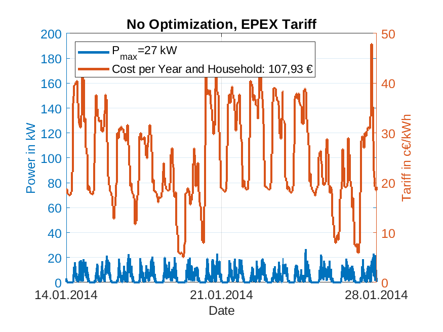
In Fig. 4a) it can be seen that an unoptimized operation leads to a good distribution of the load due to the stochastic scattering of the loading times by the users. In comparison, in Fig. 4b) one can see the fatal consequences of an uncoordinated local cost optimization. It can be clearly seen how
extreme load peaks are formed at the daily minimum price points, which reach a level that endangers grid stability.
Two basic structures can be used for the necessary coordination: A central optimization and control unit (as with Miele smart-grid Ready) or distributed optimization. In the EMWaTro project, the second variant was used for two reasons. Firstly, the structure is thus variable and individual devices can be replaced without effort. Even more important is the fact that by distributing the optimization over the devices and some central systems, the information and knowledge about the flexibilities remain on the devices and can therefore be fully exploited. Since the optimization systems have to work manufacturer-spanning, this ensures that manufacturer-specific features can be used because no secret data is transferred to a higher optimization system.
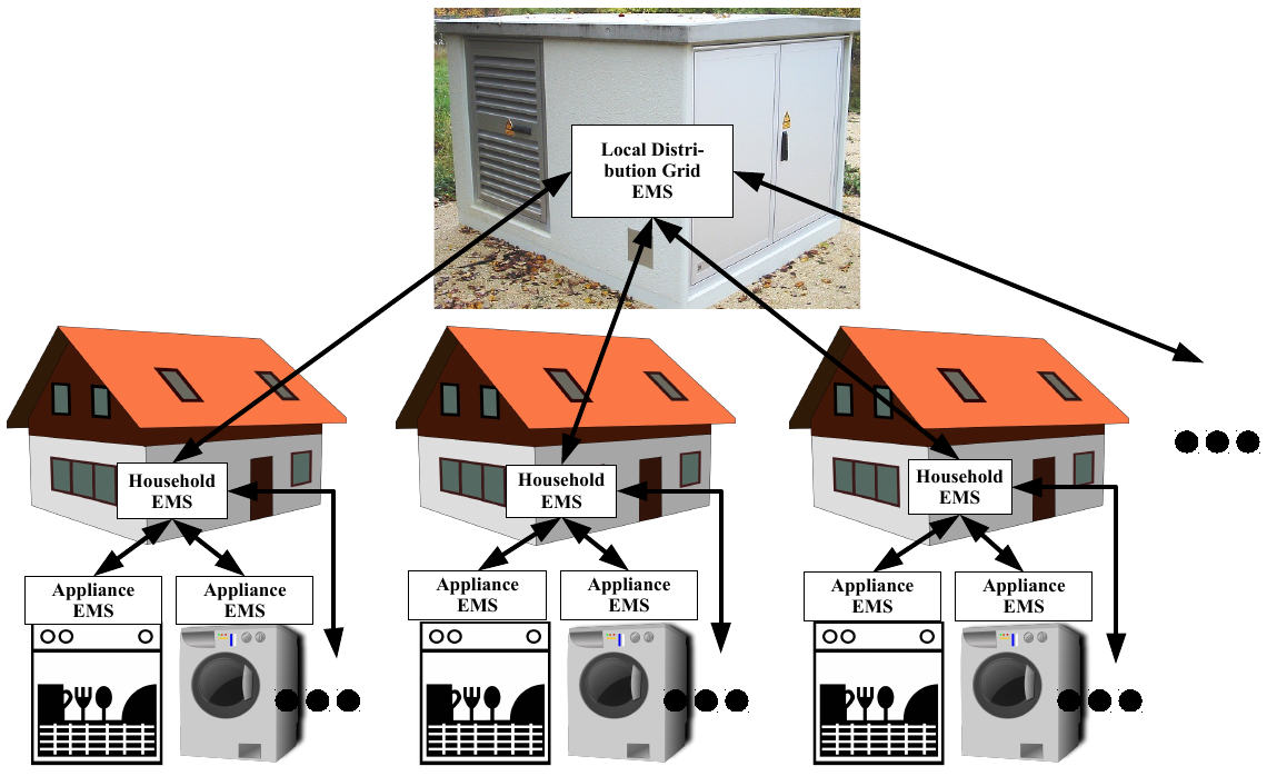
The structure of the energy management is shown in Fig. 3. It shows the three levels of energy management: appliance, household and local network energy management. At each level, pre-optimized solutions are calculated based on the available information. This means that the storage and computing effort does not increase exponentially with higher levels. The concept is explained in [2] and [3].
In addition to washer-dryers, the EMWaTro project is concerned with all household appliances that run a certain predetermined sequence program. This includes washing machines, tumble dryers and dishwashers; but also bread baking machines, ovens etc. are potentially suitable for this purpose.
The objectives of optimization differ at different levels. While the primary objective at the two in-house levels is to reduce overall costs, which causes a load shift towards excess energy supply due to the variable electricity tariff, the primary objective at the local grid level is grid stability, i.e. avoiding load peaks. This objective is also pursued at the household level as a second objective, by equalizing the burden on the household over time.
The hierarchical optimization is carried out in such a way that a certain amount of good, but locally suboptimal solutions are calculated by the devices, starting at each level, and transferred to the next higher level. From this set of offers, which represent the flexibilities in a simplified way, a more global optimization is then calculated on the next higher level via the subordinate systems. The decision is made at the highest available level and reported in the form of the selection of an offered solution through the levels up to the devices. The offers remain valid as long as the system status has not changed, e.g. by starting a program section at a certain time. In the latter case, a new quantity of offers is generated and transferred from the remaining flexibility.
At the device level, the flexibility of program-controlled devices consists in calculating a sequence of non-interruptible program parts and interruptions with a defined maximum length in such a way that the costs become minimal. As a secondary goal, the minimization of the total process duration is also taken into account. For this optimization, the Dijkstra algorithm proven in route planning is used in a slightly modified form, where the non interruptible program parts form the nodes and the pause times form the edges. The costs are allocated to the nodes and the optimization run is summed up. In contrast to the classical Dijkstra algorithm not the edge costs but the node costs are added. By additionally adding a virtual process termination node and searching for the cheapest paths to each of these nodes, the entire set of suboptimal solutions is calculated. The exact method is explained in [4].
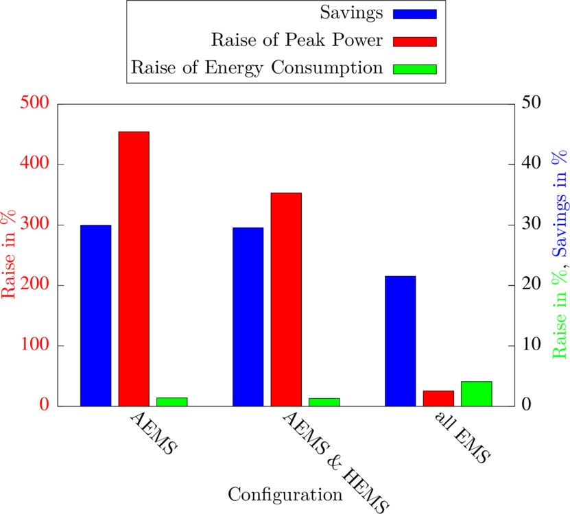
At the household level, the aim is to coordinate the offers of the individual devices in such a way that the total costs are kept as low as possible while at the same time distributing the power consumption as evenly as possible. In contrast to the function for evaluating power uniformity, the costs that are transferred from the devices with the offers are linear and can thus be superimposed. Since the complexity of the combinatorics of the bids increases exponentially with the number of connected devices, a preselection is necessary. This preselection is defined by sorting the quantities of offers and selecting the solutions that are geometrically located in a multidimensional simplex at the zero point, i.e. are relatively cheap overall. This optimization ensures that the devices are operated as close as possible to their cost optimum, but do not ensure high power peaks by simultaneous operation (usually of the heating elements). For further details please refer to [5]. The described optimization is repeated whenever, due to changes in the status of the appliances, new offers are supplied by the household appliances. As can be seen in the comparison of Fig. 4c) and Fig. 4b) as well as in Fig. 5, the optimization at household level reduces the peak load only slightly. This is due to the fact that only a small number of appliances are considered at any one time. The detailed optimization algorithm is explained in [5].
This can be remedied by optimization at the local network level, which has information about and indirect influence on a large number of devices via the offers of households. At the local network level, the minimization of costs is only an indirect goal, since billing takes place at household level. In the network, on the other hand, the maximum utilization of the infrastructure is of interest and thus the minimization of the maximum power. Since this always involves shifting loads from the cost-optimal operating time, this optimization leads to additional costs for households, which logically should also be kept low as a secondary goal. In order to avoid a costly billing and remuneration system, it is also desirable to distribute the additional costs fairly among the households. This was defined as a third optimization objective with a longer time horizon. However, the simulation has shown that stochastic scattering - even without additional consideration - results in an even fair distribution of additional costs in the long term.
Due to the high combinatorial complexity of optimization at the local network level and the lack of superposition of the load peaks, a successive algorithm was applied at this highest level. This algorithm optimizes in one step only one household by determining the offer that fits best into the sum of the already selected offers of the other households. Since the service profile and the additional costs are both totals, once the offers of one household are updated, the previously selected offer can simply be removed from the total service and the total additional costs, and there is no need for a complete reoptimization in the event of system status changes. Like comparing Fig. 4d) and Fig. 4c) and in Fig. 5 is shown, the optimization at local network level causes a reduction of the peak load to the previous level of randomly started household appliances at only low additional costs. The optimization at local network level is explained in more detail in It is an invalid source.
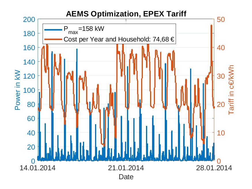
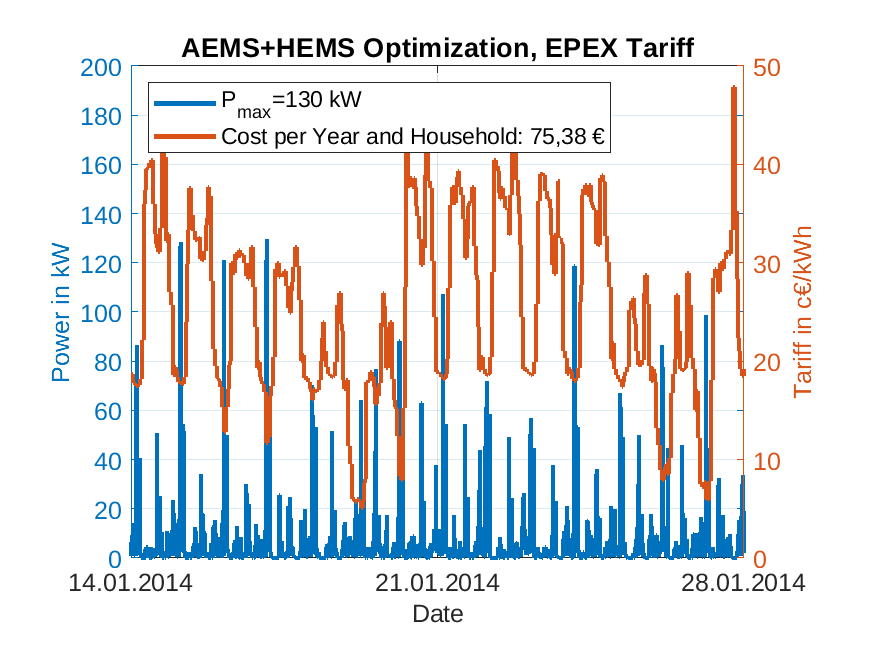
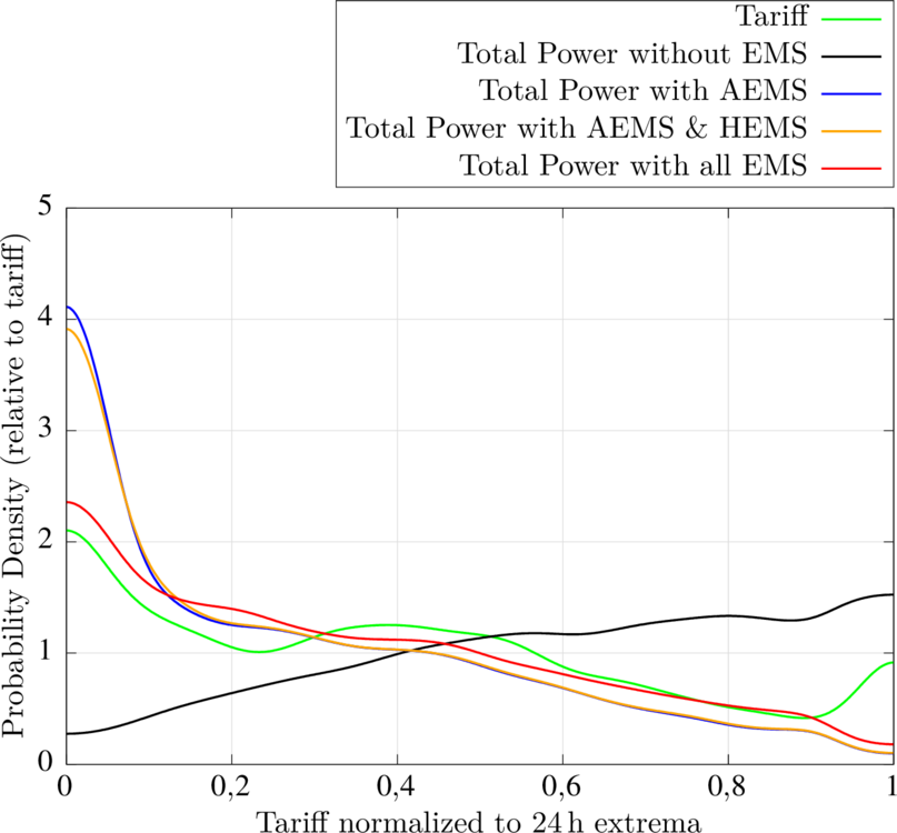
As Fig. 5 shows, the hierarchical optimization described results in cost savings while preventing a significant load peak. The real benefit for the electrical power system is shown in Fig. 6. Shown here is the frequency density distribution of the tariff level and the total output, each normalized to the daily extremes of the electricity price. The left part of the graphs is therefore the area of cheaper electricity, i.e. the area where additional loads are desired, the right part describes the times from which loads should be shifted. The graph on the left shows the status quo, where the devices are distributed evenly throughout the day due to random operation, with the power being lower at night, where the price minimum is usually currently located. With overall optimization at all levels, the overall performance is reduced over the day as a whole, even down to zero at the most expensive times. In return, the shifted loads are placed in the range of the cheapest prices.
It has thus been shown that the optimization system presented both relieves households of the price burden and contributes to a balanced power balance in a system of volatile generation without burdening the grid with peak loads. More details can be found in [7].
References:
| [1] | K. S. Stille, J. Böcker, N. Fröhleke, R. Bettentrup und I. Kaiser „Integration of Home Photovoltaic Generation into Electricity Tariff for Load Optimization“ 4th International Istanbul Smart Grid and Cities Congress, Istanbul, Türkei, 2016. |
| [2] | K. S. Stille, J. Böcker, R. Bettentrup und I. Kaiser „Concept for a Hierarchical Load Control for Domestic Appliances in Smart Grids“ 2014 IEEE International Conference on Advances in Green Energy, Thiruvananthapuram, 2014 |
| [3] | K. S. Stille, J. Böcker, R. Bettentrup und I. Kaiser „Hierarchisches Optimierungskonzept für die Laststeuerung von Haushaltsgeräten,“ ETG-Fachtagung "Von Smart Grids zu Smart Markets", Kassel, 2015 |
| [4] | K. S. Stille und J. Böcker „Local Demand Response and Load Planning System for Intelligent Domestic Appliances,“ 4th International Conference on Renewable Energy Research and Applications (ICRERA 2015), Palermo, 2015 |
| [5] | K. S. Stille, J. Böcker, N. Fröhleke, R. Bettentrup und I. Kaiser „Supervisional load optimization for households with intelligent domestic appliances“ 6th International Conference on Power Engineering, Energy and Electrical Drives (POWERENG2016), Bydgoszcz, 2016 |
| [6] | K. S. Stille und J. Böcker „Local Grid Load Coordination for Load-Shiftable Domestic Appliances in a Variable-Tariff Environment,“ 18th European Conference on Power Electronics and Applications (EPE'16 ECCE Europe), Karlsruhe, 2016 |
| [7] | K.S.Stille „Energiemanagement von Haushaltsgroßgeräten - Intelligente Lastverschiebung mit Lastspitzenvermeidung” Dissertation Paderborn University, 2018, Springer Vieweg |